
A point-mass oscillator is a basic example for understanding how inertia, stiffness and damping act together.
TONEWOOD / WOOD ACOUSTICS
From Experience to Data
Measuring, evaluating and documenting tonewood acoustics
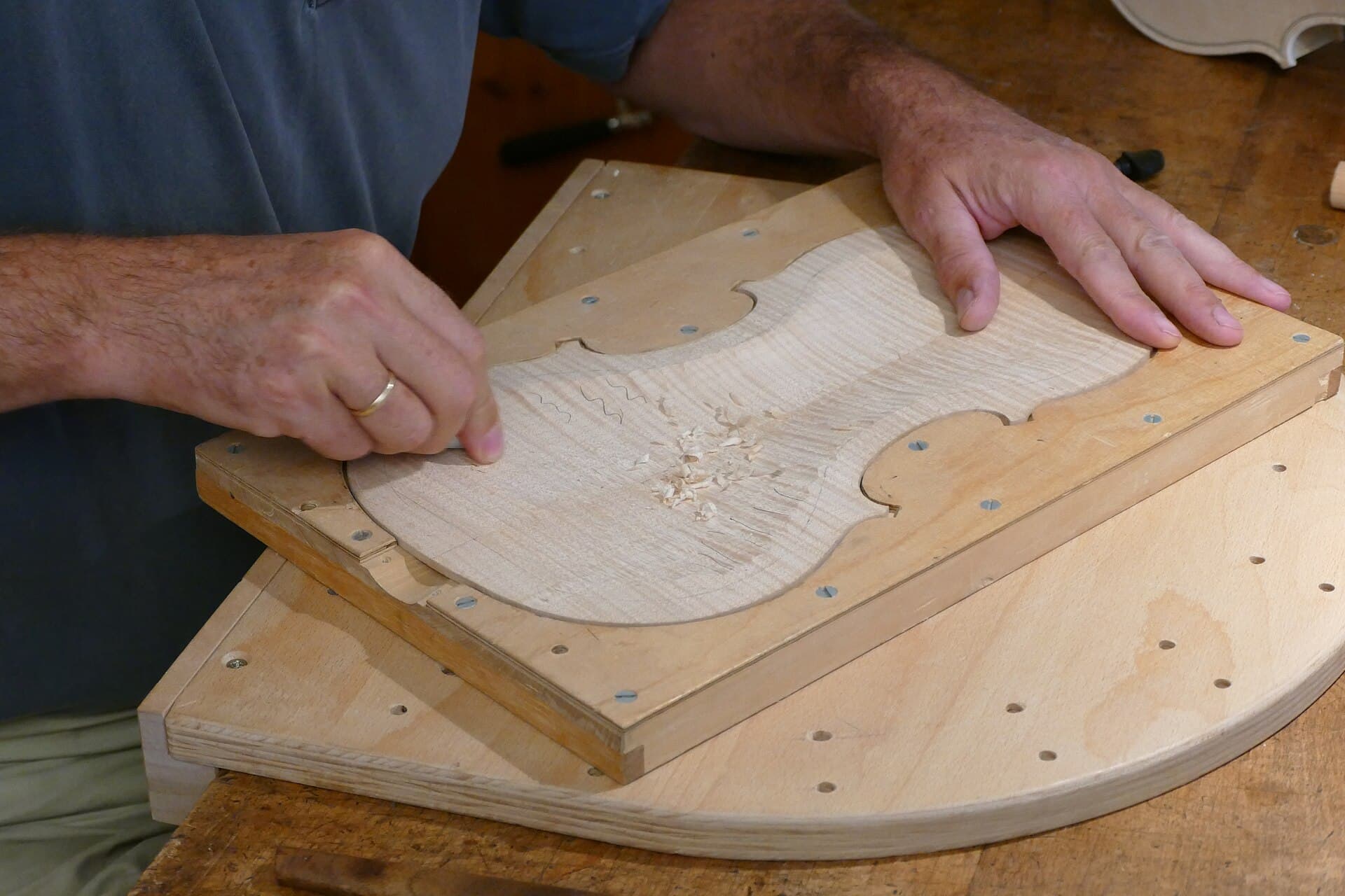
Kritzolina · Wikimedia Commons · CC BY-SA 4.0
IN THIS ARTICLE
Start reading↓Explore density, elasticity and damping, then connect acoustic indices with measurement methods and comparison conditions. Equations and interactive examples explain how data can inform material selection and why traceable records matter.
01
The whole violin
From a piece of wood to a finished violin
Materials, geometry, making and setup work together. Material measurements describe part of this system, not the finished sound on their own.
- 01
Material
- 02
Craft
Woodworking
- Free-plate arching and thickness distribution
- Coupled body modes
- Varnishing
- Setup
- 03
Nurture
- Playing
- Care
- Time
The violin body as an acoustic transformer
Violin making reconstructs the geometry, arching and thickness distribution of wood through subtractive carving, joint assembly and gluing. The resulting resonating body can be understood as an acoustic transformer with a particular frequency response. It receives string excitation through the bridge, shapes the structural response and transfers energy into sound radiation.
The Helmholtz motion of a bowed string provides an excitation signal, but the body’s material, geometry, coupling and setup shape how that excitation reaches the listener. Material properties therefore need to be understood together with the structure made from them.
The foundation of craft and the acoustic budget
Wood selection is the starting point, the foundation of the craft and the overall acoustic budget of the instrument. A maker may spend weeks, or as long as a month, on a single violin. That substantial later investment makes the starting material especially important.
Measurements provide a reference for comparing pieces and preserving the reasons for selection. They supplement the maker’s touch, listening and experience without replacing checks of grain, defects, workability or the intended instrument.
02
Experience to data
Give experience a language that can be passed on
Touch and listening offer useful observations. Measurements give those observations a shared scale and a record that can be revisited.
Sensory judgements are hard to trace
Quantifying acoustic properties does not deny the value of experience. An experienced maker may identify promising pieces quickly, but the sensations behind that choice fade with time. Years later, even when an early instrument wins a performer’s appreciation, the exact feel of its original top and back materials may be difficult to recall.
Sensory impressions cannot be preserved as reliably as recorded data. The larger purpose of measurement is therefore not merely to assign numbers, but to establish a transferable framework for describing the engineering process of violin making.
The sawtooth pattern of experience transmission
Traditional violin-making knowledge often accumulates in a sawtooth pattern. A maker spends a long time experiencing, testing and connecting plate elasticity and weight with the final voice of an instrument. This extends beyond selection to free-plate carving, plate coupling, and fine adjustments of the bridge and soundpost.
A teacher can demonstrate these actions, yet the bodily experience behind the judgement is difficult to transfer smoothly and without loss. A later generation must rediscover part of it through its own practice. The sawtooth image describes this repeated rebuilding, rather than a claim that craft makes no progress.
A shared language supports compounding knowledge
Scientific knowledge offers a contrasting model of accumulation: each result can become a starting point for the next inquiry. In this sense, knowledge can earn compound interest. When money is deposited in a bank, interest joins the principal and itself earns interest in the next period. Growth comes not only from the original deposit but also from what has already accumulated.
Knowledge can grow in the same way when methods, evidence and conclusions are expressed in a shared framework, particularly the language of mathematics. Earlier discoveries then remain available for verification and reuse, instead of leaving each generation to start again. The analogy describes cumulative reuse; it is not a measured law that all knowledge must grow exponentially.
The contrast is striking: three centuries ago, a modern electrical technology system had not yet developed; contemporary semiconductor technology includes 2 nm processes. Violin makers, meanwhile, continue to regard the Cremonese masters of three centuries ago as a formidable benchmark. The question is how each generation’s experience can become durable capital for the next.
Respect the art and introduce science
Art and science are different, and art follows its own course of development. Violin making nevertheless has an engineering and physical side as well as an artistic one. A scientific framework for that side can support knowledge accumulation without replacing artistic judgement.
Preserving measurements, methods and making experience allows later makers to revisit the evidence, discuss it and build upon earlier work.
03
Physical & acoustic properties
Physical and acoustic properties of tonewood
Density, dynamic elastic modulus and damping provide the starting quantities. Wave speed, radiation ratio, impedance and Q express particular relationships between them.
01
Start with density, elastic modulus and damping; then connect the acoustic indices.
THREE PROPERTIES, ONE OSCILLATOR
Mass, stiffness and decay, together.
One equation connects inertia, damping and stiffness.
++
x is displacement from equilibrium, ẋ is velocity and ẍ is acceleration. After release there is no sustained external driving force; the three terms satisfy this equation of motion.
Inertia: Newton’s second law
Newton’s second law, ΣF = mẍ, relates net force to acceleration. At fixed volume, density enters the inertia term through m = ρV.
Damping: dissipation and the second law
Passive damping irreversibly dissipates mechanical energy, consistent with the second law of thermodynamics. Here it is represented by the equivalent viscous force −bẋ, with b ≥ 0.
Stiffness: constitutive relation and Hooke’s law
Hooke’s law is a linear elastic constitutive relation. The restoring force is −kx; at fixed geometry, elastic modulus E sets equivalent stiffness k.
DisplacementDecay envelopeCurrent displacement
Synchronized motion and cursor · 100× slower
Density → mass m → inertia term, at fixed volume.
Modulus → stiffness k → stiffness term, at fixed geometry.
Loss factor η → equivalent damping b → damping term.
Equivalent mass m = ρV4.20 g
Undamped natural frequency f₀101.6 Hz
Quality factor Q ≈ 1/η111.1
Model and equations
The equivalent volume is fixed at V = 10 cm³. The reference frequency is 100 Hz at ρ = 400 kg/m³ and E = 12 GPa. Parameter changes restart the release at x/x₀ = 1 with zero initial velocity. The loss factor is represented by equivalent viscous damping near a single resonance.
The chart uses physical time. One second of playback advances the model by 10 ms; the full 400 ms response plays over 40 seconds.
COMSOL · About damping ↗UT Austin · Damped harmonic oscillation ↗3.2ρ
Density
Mass per unit volume: a way to quantify light and heavy.
kg/m³
3.3E
Dynamic elastic modulus
Material stiffness during vibration, distinguished from the stiffness of a shaped plate.
GPa
3.4η
Damping
Describes vibrational energy loss using the loss factor η. At the same frequency, a larger loss factor means faster decay.
Dimensionless
Compare the indices of three materials
Density, dynamic elastic modulus and damping describe different parts of a material’s behaviour. In the weak-damping approximation, Q ≈ 1/η provides another way to express loss. Three illustrative pieces can be used to examine what these quantities mean for soundboard selection.
A has the lowest density, while C has the highest modulus and Q. B lies between them in all three inputs. Their Q values, 120, 121 and 122, are close. Looking at any one quantity alone does not yet resolve the material choice.
The basic parameters contain the information needed for the following calculations. The remaining question is how their combined effects serve a particular making goal: whether extra stiffness compensates for extra inertia, how lightness and stiffness can be considered together, and which quantity relates stress to particle velocity in a traveling wave.
Wave speed, radiation ratio and characteristic impedance answer these different questions, with Q describing loss. These derived indices do not add independent material information; they reorganize it into comparisons that are easier to interpret.
Switching the comparison index shows why the ordering can change. A higher value is not always better, particularly for characteristic impedance. Intended use and comparable measurement conditions remain necessary.
Material A
Loading 3D model…
- Density ρ
- 360kg/m³
- Dynamic modulus E
- 12GPa
- Q
- 120dimensionless
Material B
Loading 3D model…
- Density ρ
- 400kg/m³
- Dynamic modulus E
- 15GPa
- Q
- 121dimensionless
Material C
Loading 3D model…
- Density ρ
- 450kg/m³
- Dynamic modulus E
- 16GPa
- Q
- 122dimensionless
Make a choice, then explore another perspective.
How do stiffness and inertia balance?
B has the highest wave speed, with C close behind.
In the one-dimensional model, both modulus and density matter. Relative to A, B’s wave speed is 6.1% higher and C’s is 3.3% higher. Modulus alone does not describe this balance.
Illustrative data · Same direction, comparable frequencies and measurement conditions. A low-loss one-dimensional longitudinal model is used, with Q dominated by material loss. Bars compare values, not quality scores.
02
Four derived acoustic indices
Wave speed, radiation ratio and characteristic impedance combine E and ρ in different ways; quality factor Q describes vibrational energy loss.
3.5c
Wave speed
In the one-dimensional model, wave speed reflects stiffness relative to density.
m/s
3.6R
Acoustic radiation ratio
Wave speed divided by density: a material index connecting lightness and stiffness.
m⁴/(kg·s)
3.7Z
Characteristic impedance
Density times wave speed: a material quantity used to discuss wave transmission.
Pa·s/m
3.8Q
Quality factor
Measures vibrational energy retention. At the same frequency, higher Q means lower loss and slower decay; the relation below assumes weak damping.
Dimensionless
3.9 / Property reference+
| Property | Formula | Unit |
|---|---|---|
| Density | kg/m³ | |
| Dynamic elastic modulus | GPa | |
| Damping | Dimensionless | |
| Wave speed | m/s | |
| Acoustic radiation ratio | m⁴/(kg·s) | |
| Characteristic impedance | Pa·s/m | |
| Quality factor | Dimensionless |
04
Measurement methods
Measure stiffness and vibrational loss
Resonance frequency and specimen geometry can be used to estimate dynamic modulus; the decay of an identified mode can be used to estimate damping and Q.
4.1–4.3
How can we measure elastic modulus?
Static testing
Apply a known load and measure strain in the elastic range.
Ultrasonic testing
Measure pulse travel time over a known distance; infer modulus using an appropriate wave model.
Impulse excitation
Measure geometry, density and the frequency of an identified bending mode, then solve for the dynamic elastic modulus.
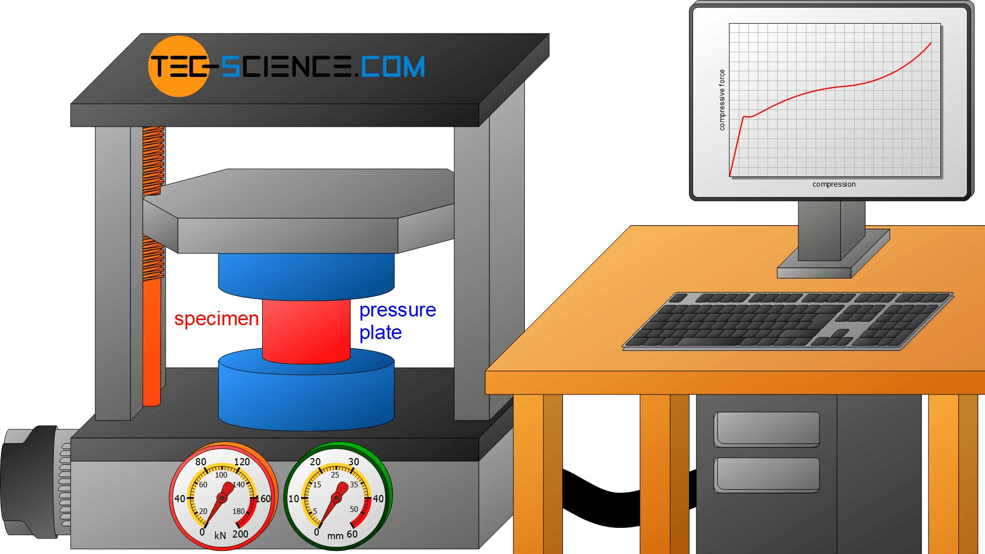 Illustration of the compression-testing principle.
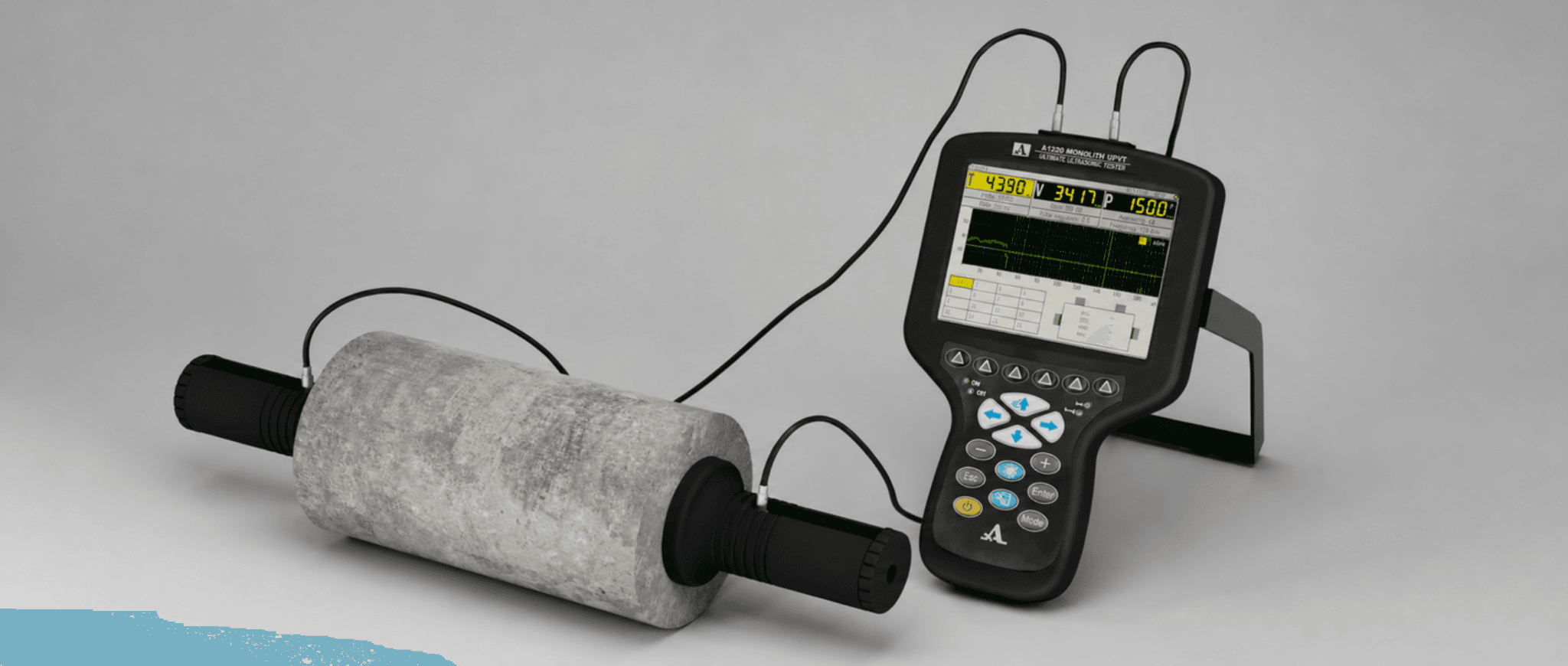 Illustration of ultrasonic transmission measurement.
4.3
From resonance frequency to elastic modulus.
For a given geometry, elastic modulus and density, the frequency of a specified vibration mode is determined. Measuring the geometry, density and frequency of that mode lets us work backwards through the same model to estimate the elastic modulus.
Forward: material and geometry set frequency
Dynamic modulus E′ + density ρ + geometryMode frequency fₙ
Inverse: measured frequency gives modulus
Measured geometry + density ρ + mode frequency fₙDynamic modulus E′
Identify the bending mode and match the boundary conditions and geometry model. The equations shown assume a uniform, slender, constant-section free–free beam.
Loading 3D model…
Theory: from beam vibration to dynamic elastic modulus
Inverting a free beam’s impact-excited bending resonance to obtain dynamic elastic modulus starts from the Euler–Bernoulli equation for free bending vibration:
Here w(x,t) is transverse displacement. A harmonic modal solution with free–free boundary conditions gives the frequency and inverse relations:
The nonzero free–free characteristic roots satisfy cos βₙ cosh βₙ = 1. The first non-rigid bending mode has β₁ ≈ 4.73004, so inversion using its frequency f₁ gives: Woodpedia: mode shapes and βₙ for different boundaries ↗
Formula parameters
| Symbol | Meaning | SI unit |
|---|---|---|
| Dynamic flexural Young’s modulus | ||
| Natural resonance frequency of the first non-rigid bending mode | ||
| Total specimen beam length | ||
| Specimen mass, measured by weighing | ||
| Specimen volume, calculated from measured dimensions | ||
| Material density | ||
| Specimen cross-sectional area | ||
| Second moment of area about the centroidal axis appropriate to the bending direction | ||
| Dimensionless characteristic root set by boundary conditions and mode number; β₁ ≈ 4.73004 for the first free–free bending mode |
(1) Trapezoidal section: wedge blanks
For an isosceles trapezoidal blank section of width a, thin-edge thickness h₁ and thick-edge thickness h₂, the second moments of area about its orthogonal centroidal principal axes are:
For the illustrated first flatwise bending mode, displacement is in the thickness direction and bending is about y_c. Thus, inversion of the longitudinal dynamic modulus uses I = I_yc. Combining this with the trapezoidal area gives:
Substitute A / I_yc into the Euler–Bernoulli inverse relation:
Use β₁ = 4.73004… for the first free–free bending mode (β₁⁴ ≈ 500.5639). In practice, we weigh the specimen and measure its dimensions. Write density as mass M divided by volume, and express that volume using the measured wedge dimensions:
Insert the measured mass M, length L, width a, edge thicknesses h₁ and h₂, and first bending frequency f₁ directly. Use kg, metres and Hz to obtain E′ in Pa.
(2) Rectangular section: constant-thickness strips
When h₁ = h₂ = h, the trapezoid becomes a rectangle: A = ah and I_yc = ah³ / 12. The formula then reduces to the classical rectangular-strip expression:
Both coefficients use β₁ = 4.7300407449…: 96π² / β₁⁴ ≈ 1.8928293 and 48π² / β₁⁴ ≈ 0.9464147. Use metres, kg/m³ and Hz throughout to obtain E′ in Pa.
(3) Thickness and shear correction: Timoshenko beam factor T′
As the thickness-to-length ratio h/L increases, transverse shear deformation and rotary inertia become more significant. They lower the resonance frequency relative to the elementary Euler–Bernoulli prediction, so inversion without correction underestimates the dynamic modulus. Multiply the preceding inverse relation by the thickness correction factor T′:
The correction accounts for shear and rotary-inertia effects considered in Timoshenko beam theory, using the ASTM E1876 / Pickett form. It is denoted T′ here and corresponds to the standard’s rectangular-beam factor T₁; μ is Poisson’s ratio. The full expression is:
For a rectangular strip, h is its actual thickness in the bending direction. For the preceding isosceles trapezoidal wedge, ToneWood substitutes an equivalent thickness matching I/A:
Engineering approximation: μ ≈ 0.30, neglecting fourth-order terms
For a small thickness-to-length ratio and an assumed μ ≈ 0.30, the quadratic coefficient is approximately 7.214, giving:
This engineering approximation assumes a Poisson’s ratio. ASTM’s slender rectangular-beam simplification is T₁ = 1 + 6.585(h/L)² for L/h ≥ 20, a different approximation. State the assumed Poisson’s ratio when it is unknown.
ToneWood’s calculation assumes μ = 0.30 and evaluates the full correction. Applying the rectangular-beam expression with an equivalent thickness to orthotropic wooden wedges is an engineering extension whose applicability needs validation against reference specimens.
Geometry and vibration assumptions
The derivation assumes a slender beam of constant cross-section, uniform density and elastic properties along its length, approximately free ends, and identification of the first non-rigid bending mode in the chosen direction. When the beam length follows the grain, E′ is the dynamic flexural Young’s modulus in that direction.
The illustrated wedge varies in thickness across its width, not along its length. These section moments apply to the shown isosceles trapezoid and axes. A right-trapezoidal section, a longitudinal taper or a different bending direction requires the appropriate section moments and beam model. Short, thick specimens also need shear and rotary-inertia corrections.
Clamped, supported and free differ.
Boundary conditions determine mode shapes and characteristic roots. Support and holding positions must suit the measured mode.
Short, thick specimens need care.
Shear deformation and rotary inertia matter more as thickness-to-length ratio grows. The model and correction must suit the specimen.
Measure thickness as carefully as frequency.
Length, thickness, mass and frequency all affect the result. Thickness is especially sensitive; the estimated Poisson ratio enters the correction.
How does ToneWood measure damping and Q?
SupplementThe same tap serves two measurements: frequency, geometry and density give elastic modulus; the decay over time gives damping and Q.
Locate the mode in the same tap
An FFT identifies the target mode frequency f₀ in the tap recording. A bandpass filter then isolates the response around that frequency.
Extract the usable decay envelope
A moving RMS window extracts the amplitude envelope. The impact transient is skipped, the recording tail estimates the noise floor, and the usable decay above that threshold is retained.
Find the decay rate from a logarithmic fit
A single mode has an approximately exponential amplitude decay. Fitting the natural logarithm of its envelope against time gives the slope −γ and hence the decay rate.
Convert the decay rate to loss factor and Q
For a single mode under a linear, light-damping approximation, its frequency f₀ and decay rate give the loss factor tan δ and quality factor Q. At the same frequency, slower decay means higher Q.
The dashed curves enclose the oscillation; only the positive envelope is log-transformed on the right. Gold points mark the same sampling times in both plots. Illustration of the principle, not App measurement data.
Fit the amplitude envelope
Light-damping conversion
Support, sound radiation, surroundings and filtering can affect the measured modal decay. Compare materials using the same mode, direction and measurement conditions.
Theory: Euphonics · Vibration damping ↗05
Indices and making decisions
Interpret acoustic indices in the context of making
Once the basic vibrational properties have been measured, the comparison can move from raw material to violin plates. Wave speed, radiation ratio and characteristic impedance then help interpret thickness, mass and structural response under stated conditions.
At the same target frequency, why do thickness and mass differ?
Acoustic measurements become useful when brought back into the making process. During thinning, plate mass and modal frequency are recorded together, because thickness, mass and frequency all change as material is removed.
A plate may reach the intended frequency while still relatively thick or heavy, while another reaches that frequency only after being made thinner. For example, a top plate may reach Mode 5 = 350 Hz yet still weigh 80 g. Further thinning may reduce its mass to the intended range but also lower its modal frequency below the target. These are illustrative making values, not universal targets.
Even when a workshop uses similar models and archings, this trade-off can recur. The practical question is whether measurements can provide some basis, before carving starts, for anticipating the likely final thickness and mass. Wave speed, radiation ratio and characteristic impedance offer different perspectives on that question under stated comparison assumptions.
Making exampleMode 5 = 350 Hz
Mass: sometimes 60-something g, sometimes 80-something gThickness: sometimes 2.3 mm, sometimes 2.8 mm
At the same 350 Hz, mass and thickness can each differ. Keep thinning, or stop?
The frequency, masses and thicknesses are discussion examples, not universal plate targets.
Wave speed: frequency at equal thickness, thickness at equal frequency.
Longitudinal wave
Slowed 30,000× · displacement enlargedIn a longitudinal wave, particles vibrate parallel to the direction of wave propagation.
For a soundboard, longitudinal motion within the plane usually drives the surrounding air only weakly.
Model and references
Longitudinal motion uses a one-dimensional slender-rod approximation; bending uses a rectangular Euler–Bernoulli beam. Aₛ is cross-sectional area and I its second moment, with I/Aₛ = h²/12. The transverse wave here is a bending wave; bulk shear waves depend on shear modulus. Real plates also involve anisotropy, arching and thickness distribution.
The final step uses reference plate shapes for Mode 1–5 rather than the beam frequencies. Frequency scaling assumes comparable elastic ratios; these teaching shapes are not eigenvalue solutions for a real arched plate.
Euphonics · Bending beams ↗Penn State · Wave motion ↗We have considered thickness. Why can mass still differ?
How does radiation ratio R bring mass into the comparison?
Frequency scales with overall thickness and wave speed in this bending model.
With effective area A fixed, express thickness using mass and density.
Substitute thickness and collect c/ρ.
At fixed area, mass and R together set the frequency scale.
1 / 4
Characteristic impedance Z: choosing between equal-R materials.
Another index is characteristic impedance Z: density multiplied by wave speed.
Return to the previous question. Under the simplified comparison, two materials with equal R reach Mode 5 = 350 Hz at the same mass, but one plate can be thinner and the other needs to be thicker. Which would you choose?
At this point, I would use Z to discuss style and personal preferences rather than rank materials as good or bad.
Compare these two illustrative parameter sets, both with R = 14 m⁴/(kg·s).
Lower Z
Lower density and wave speed → a relatively thicker plate
- Density ρ
- 350 kg/m³
- Longitudinal speed c
- 4,900 m/s
Characteristic impedance Z = ρc1.715 MRayl
350 × 4,900 = 1,715,000 kg/(m²·s)
Playing feel: I would hope for a gentle onset, with the sound opening under lighter bow pressure and an approachable response.
Tone: I would look for warmth, roundness and an enveloping quality, while checking whether strong playing reaches a dynamic limit too early or feels like pressing into cotton wool.
Higher Z
Higher density and wave speed → a relatively thinner plate
- Density ρ
- ≈ 414.29 kg/m³
- Longitudinal speed c
- 5,800 m/s
Characteristic impedance Z = ρc2.403 MRayl
414.29 × 5,800 ≈ 2,402,857 kg/(m²·s)
Playing feel: I would look for a clear sense of resistance and check how much dynamic room remains under greater bow pressure.
Tone: I would hope for distinct articulation, focus, line and projection, while watching for a sound that is too tight or cold, or demands greater control.
R is identical, while the higher-Z material has about 1.40 times the characteristic impedance.
These parameters illustrate plausible soundboard-material values; they are not a measured pair.
These are experience-based selection ideas to test against the actual plate structure and playing results. Bring your own preferences to the material map below.
Return to the material map: choose two points and compare.
Material acoustic properties
Select a point in either chart to see its measurements- ρDensity
- —kg/m³
- cWave speed
- —m/s
- EElastic modulus
- —GPa
- QQuality factor
- —dimensionless
- RRadiation ratio
- —m⁴/(kg·s)
- ZCharacteristic impedance
- —MRayl
Loading the lab…
5.6
Express material preferences in a combined score
Wave speed helps interpret thickness, radiation ratio helps compare mass, and characteristic impedance provides a way to discuss material preferences. A combined score brings these selection considerations onto a reference scale. The example starts with R and Q, then returns to materials A, B and C to show how an explicit preference changes their comparison. It is a selection model, not a universal definition of wood quality.
An example soundboard Acoustic Score model
The baseline normalizes R and Q by their reference values, multiplies those ratios, and scales the result by 100. In the longitudinal one-dimensional approximation, c = √(E/ρ) and R = c/ρ, so expanding R gives a modulus exponent of 1/2 and a density exponent of −3/2. Q enters linearly to include vibrational loss: with the other inputs fixed, a ten-percent increase in Q raises this score by ten percent.
The references are 12 GPa, 420 kg/m³ and Q = 120. The reference material scores 100, but 100 is not a ceiling. The formula reorganizes existing material information; choosing it as a selection score expresses a preference for radiation ratio together with low loss. Its usefulness must still be assessed against making goals and outcomes.
- Reference radiation ratio
- 12.7267 m⁴/(kg·s)
- Reference density
- 420 kg/m³
- Reference Q
- 120 dimensionless
Rₗ = cₗ/ρ and Qₗ is the longitudinal vibration quality factor. R₀ follows from E₀ = 12 GPa and ρ₀ = 420 kg/m³; calculations use its unrounded value. The reference scores 100, not a ceiling or percentile.
Stiffness contribution
With the other inputs fixed, a higher longitudinal modulus raises the score. The square root follows from the relation between wave speed and modulus.
E +10% → score about +4.9%Starting with radiation ratio
Radiation ratio Rₗ = cₗ/ρ gives a density exponent of −3/2. At the same modulus and Q, the baseline favours lower density.
ρ −10% → score about +17.1%Including vibrational loss
Under comparable measurement conditions, higher Q indicates lower vibrational loss. The recommended formula includes normalized Q linearly.
Q +10% → score +10.0%These comparisons use the baseline and change one input at a time. Factors multiply; exponents express relative sensitivity, not additive percentage weights.
Express selection choices through impedance preference
At α = −1.50 the score follows normalized R × Q. At equal R and Q, moving toward −1.75 favours lower characteristic impedance; moving toward −1.25 favours higher impedance. This is a gentle local preference around the balanced baseline, not a change to saved database scores.
The exponent expresses a preference, not a universal optimum. At the same Eₗ and Qₗ, lower density still scores higher throughout this range. The preference for higher wave speed applies when Rₗ is held constant.
What scores do the example materials A, B and C from Part 3 receive?
Move the α slider to see how the three scores and their ranking change. The reference material always scores 100.
−1.75
Lower Z−1.50
Balanced−1.25
Higher Z
Lower Z−1.50
Balanced−1.25
Higher Z
Left: a gentle, full target; right: a bright, focused, projecting target. These describe selection goals, not predicted violin tone. Only α changes; material measurements, references and linear Q remain fixed.
Material A
126.0Recommended baseline score
Eₗ = 12 GPa
ρ = 360 kg/m³ · Qₗ = 120
Change from baseline: 0.0 points
Material B
121.3Recommended baseline score
Eₗ = 15 GPa
ρ = 400 kg/m³ · Qₗ = 121
Change from baseline: 0.0 points
Material C
105.9Recommended baseline score
Eₗ = 16 GPa
ρ = 450 kg/m³ · Qₗ = 122
Change from baseline: 0.0 points
At α = -1.50, the scores from highest to lowest are A (126.0), B (121.3), C (105.9).
When the impedance preference changes, Q still enters linearly. These scores express a selection preference under the stated formula; they neither determine finished sound quality nor measure its percentage improvement.
Moving α does not change the wood. What changes is the local characteristic-impedance preference around the R × Q baseline. At equal R and Q, α below −1.50 favours lower Z and α above it favours higher Z. A score therefore needs its formula, comparison conditions and intended use alongside it.
Whether that preference helps produce the intended violin cannot be answered by the score alone. The original reasoning needs to be recorded together with the later making and playing results. This turns an isolated number into a decision that can be reviewed, compared and revised as material records accumulate.
Further reading: plate bending impedance and comparison assumptions
Plate bending impedance Zᵦ
h is thickness, M is plate mass and f₅ is Mode 5 frequency; ∝ denotes scaling, not numerical equality.
Measures resistance to vibrational velocity under a driving force. The actual response also depends on frequency, damping and driving position.
Zᵦ is a plate bending-impedance scale; material characteristic impedance is z = ρc. They describe different quantities.
The thin-plate scaling relations assume the same outline, area, boundary conditions and thickness-profile shape, with a consistently defined directional or effective E. Real plates also depend on anisotropy, arching and local thickness.
Reference: Barlow · Materials Selection for Musical Instruments (1997) ↗06
Records and shared data
From a measurement to a traceable material record
The lasting value of a measurement depends on the identity, conditions and evidence kept with it, and on the comparisons that become possible over time.
- 01
A reference for selection and a scale for experience
Measurement gives beginners and experienced makers different but complementary forms of support. For a beginner, comparing a piece with a material database provides a starting reference: what are its characteristics, and how does it differ from other pieces? Measurements can be considered together with touch and listening as judgement develops.
For an experienced maker, measurement gives established intuition a scale. A piece may already feel promising, but its particular strengths and suitability for an intended violin can be described more precisely. Connecting impressions with quantities makes experience easier to compare, share, preserve and test in later making.
- 02
Design controlled experiments
A phone-based laboratory can support experiments designed around everyday making questions. The same piece can be measured at different moisture contents, allowing elastic modulus, wave speed and Q to be compared after each moisture state has stabilized.
Sealing and varnishing can be studied on the same thin plate by recording mass, resonance frequencies and Q before and after each treatment, while keeping the method and moisture conditions comparable. These changes can then be considered together with what is heard and felt.
Arching offers another question: select materials with similar acoustic properties, hold the violin model and thickness plan as consistent as possible, and compare different archings while documenting remaining material differences. Such accumulated comparisons can also inform how much acoustic allowance to leave during free-plate carving for subsequent sealing and varnishing.
- 03
Build on every making experience
Measurements become more useful when linked to the making process and the finished instrument’s performance. Retain the selection rationale, arching and thickness decisions, adjustments and playing observations as a connected record.
After completion and use, revisit the original choice in light of the result. Repeated comparison helps identify which judgements were supported and which need revision. One violin does not isolate material effects from craft and setup, but a growing set of traceable records can make the next choice better informed.
- 04
Trace every violin’s material story
Assign a stable material ID and keep physical and acoustic indices together with the material state and measurement conditions. Dimensions, mass, direction, moisture, temperature, test method, recordings, mode identification, repeat measurements and algorithm versions all provide context for later review.
Link that ID to the particular violin so that selection, making and playing observations remain connected. Years later, the record can answer not only which material was used, but also why it was selected, how it was worked and what was learned from the finished instrument. A shared database can support comparison within the same use and part while making missing data and biased samples easier to identify.